General matrix notation of a VAR(p)

This page just shows the details for different matrix notations of a VAR(p) process with k variables.

Contents

Var(p)

y_{t}=c %2B A_{1}y_{t-1} %2B A_{2}y_{t-2} %2B \cdots %2B A_{p}y_{t-p} %2B e_{t},

Where each y_{i} is a k x 1 vector and each A_{i} is a k x k matrix.

Large matrix notation

\begin{bmatrix}y_{1,t} \\ y_{2,t}\\ \vdots \\ y_{k,t}\end{bmatrix}=\begin{bmatrix}c_{1} \\ c_{2}\\ \vdots \\ c_{k}\end{bmatrix}%2B
\begin{bmatrix}
a_{1,1}^1&a_{1,2}^1 & \cdots & a_{1,k}^1\\ 
a_{2,1}^1&a_{2,2}^1 & \cdots & a_{2,k}^1\\ 
\vdots& \vdots& \ddots& \vdots\\
a_{k,1}^1&a_{k,2}^1 & \cdots & a_{k,k}^1
\end{bmatrix}
\begin{bmatrix}y_{1,t-1} \\ y_{2,t-1}\\ \vdots \\ y_{k,t-1}\end{bmatrix}
%2B \cdots %2B
\begin{bmatrix}
a_{1,1}^p&a_{1,2}^p & \cdots & a_{1,k}^p\\ 
a_{2,1}^p&a_{2,2}^p & \cdots & a_{2,k}^p\\ 
\vdots& \vdots& \ddots& \vdots\\
a_{k,1}^p&a_{k,2}^p & \cdots & a_{k,k}^p
\end{bmatrix}
\begin{bmatrix}y_{1,t-p} \\ y_{2,t-p}\\ \vdots \\ y_{k,t-p}\end{bmatrix}

 %2B \begin{bmatrix}e_{1,t} \\ e_{2,t}\\ \vdots \\ e_{k,t}\end{bmatrix}

Equation by equation notation

Rewriting the y variables one to one gives:

y_{1,t} = c_{1} %2B a_{1,1}^1y_{1,t-1} %2B a_{1,2}^1y_{2,t-1} %2B\cdots %2B a_{1,k}^1y_{k,t-1}%2B\cdots%2Ba_{1,1}^py_{1,t-p}%2Ba_{1,2}^py_{2,t-p}%2B \cdots %2Ba_{1,k}^py_{k,t-p} %2B e_{1,t}\,

y_{2,t} = c_{2} %2B a_{2,1}^1y_{1,t-1} %2B a_{2,2}^1y_{2,t-1} %2B\cdots %2B a_{2,k}^1y_{k,t-1}%2B\cdots%2Ba_{2,1}^py_{1,t-p}%2Ba_{2,2}^py_{2,t-p}%2B \cdots %2Ba_{2,k}^py_{k,t-p} %2B e_{2,t}\,

\qquad\vdots

y_{k,t} = c_{k} %2B a_{k,1}^1y_{1,t-1} %2B a_{k,2}^1y_{2,t-1} %2B\cdots %2B a_{k,k}^1y_{k,t-1}%2B\cdots%2Ba_{k,1}^py_{1,t-p}%2Ba_{k,2}^py_{2,t-p}%2B \cdots %2Ba_{k,k}^py_{k,t-p} %2B e_{k,t}\,

Concise matrix notation

One can rewrite a VAR(p) with k variables in a general way which includes T+1 observations y_{0} through y_{T}

 Y=BZ %2BU \,

Where:

 Y=
\begin{bmatrix}y_{p} & y_{p%2B1} & \cdots & y_{T}\end{bmatrix} =
\begin{bmatrix}y_{1,p} & y_{1,p%2B1} & \cdots & y_{1,T} \\ y_{2,p} &y_{2,p%2B1} & \cdots & y_{2,T}\\
\vdots& \vdots &\vdots &\vdots \\  y_{k,p} &y_{k,p%2B1} & \cdots & y_{k,T}\end{bmatrix}
 B=
\begin{bmatrix} c & A_{1} & A_{2} & \cdots & A_{p} \end{bmatrix} = 
\begin{bmatrix}
c_{1} & a_{1,1}^1&a_{1,2}^1 & \cdots & a_{1,k}^1 &\cdots & a_{1,1}^p&a_{1,2}^p & \cdots & a_{1,k}^p\\ 
c_{2} & a_{2,1}^1&a_{2,2}^1 & \cdots & a_{2,k}^1 &\cdots & a_{2,1}^p&a_{2,2}^p & \cdots & a_{2,k}^p \\ 
\vdots & \vdots& \vdots& \ddots& \vdots & \cdots & \vdots& \vdots& \ddots& \vdots\\
c_{k} & a_{k,1}^1&a_{k,2}^1 & \cdots & a_{k,k}^1 &\cdots & a_{k,1}^p&a_{k,2}^p & \cdots & a_{k,k}^p 
\end{bmatrix}

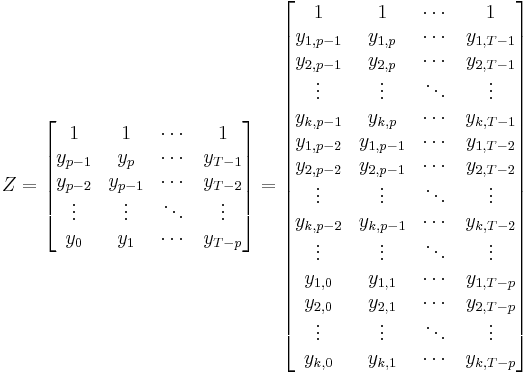
Z=
\begin{bmatrix}
1 & 1 & \cdots & 1 \\
y_{p-1} & y_{p} & \cdots & y_{T-1}\\
y_{p-2} & y_{p-1} & \cdots & y_{T-2}\\
\vdots & \vdots & \ddots & \vdots\\
y_{0} & y_{1} & \cdots & y_{T-p}
\end{bmatrix} =
\begin{bmatrix}
1 & 1 & \cdots & 1 \\
y_{1,p-1} & y_{1,p} & \cdots & y_{1,T-1} \\
y_{2,p-1} & y_{2,p} & \cdots & y_{2,T-1} \\
\vdots & \vdots & \ddots & \vdots\\
y_{k,p-1} & y_{k,p} & \cdots & y_{k,T-1} \\
y_{1,p-2} & y_{1,p-1} & \cdots & y_{1,T-2} \\
y_{2,p-2} & y_{2,p-1} & \cdots & y_{2,T-2} \\
\vdots & \vdots & \ddots & \vdots\\
y_{k,p-2} & y_{k,p-1} & \cdots & y_{k,T-2} \\
\vdots & \vdots & \ddots & \vdots\\
y_{1,0} & y_{1,1} & \cdots & y_{1,T-p} \\
y_{2,0} & y_{2,1} & \cdots & y_{2,T-p} \\
\vdots & \vdots & \ddots & \vdots\\
y_{k,0} & y_{k,1} & \cdots & y_{k,T-p} 
\end{bmatrix}

and

U= 
\begin{bmatrix}
e_{p} & e_{p%2B1} & \cdots & e_{T}
\end{bmatrix}=
\begin{bmatrix}
e_{1,p} & e_{1,p%2B1} & \cdots & e_{1,T} \\
e_{2,p} & e_{2,p%2B1} & \cdots & e_{2,T} \\
\vdots & \vdots & \ddots & \vdots \\
e_{k,p} & e_{k,p%2B1} & \cdots & e_{k,T} 
\end{bmatrix}.

One can then solve for the coefficient matrix B (e.g. using an ordinary least squares estimation of  Y \approx BZ)

References